When Accuracy Lies: Imbalanced Data Counterfeit Metrics
08 September 2025
What if I told you that a model with 86% accuracy is actually worse than random guessing? In this post, I’ll show you how accuracy can be a dangerous lie when your data is imbalanced.
In the world of machine learning, not all metrics are created equal, especially when the data used for model building is imbalanced. Probably we have all seen models boast 90% or even 99% accuracy. But what if that performance is just mirroring the data distribution?
I recently worked on a classifier for chemical property predictions, and this experience reminded me why accuracy alone can be dangerously misleading. Let me walk you through a guided tour of metrics that actually matter, and most importantly why.
The Counterfeit Comfort of Accuracy
Imagine you’re building an ML model for a common task in pharmaceutical research: predicting whether chemical compounds will bind to specific protein targets. This prediction could help identify promising drug candidates early in the development process.
In a typical drug discovery dataset, you’ll find a striking imbalance. For example, we may find that out of 10,000 compounds tested against a protein target, only about 300 (3%) show any binding activity at all. The remaining 9,700 compounds (97%) show no binding. Which is, by the way, the harsh and sad reality of drug discovery: the vast majority of compounds simply don’t work. :(
Now, here’s where accuracy becomes a deceptive trap. Consider a model that lazily predicts every single compound as “non-binding.” It would achieve an impressive 97% accuracy score, but it would be completely useless in practice. Such a model would never identify a single promising drug candidate, defeating the entire purpose of our prediction task!
When building models with skewed data like this, accuracy is as helpful as a broken compass!
What are the options when working with imbalanced data?
Our options for evaluating models on imbalanced data go beyond just accuracy. Here are the key metrics we should consider:
- Precision
- Recall
- F1-Score
- ROC-AUC (Receiver Operating Characteristic AUC)
- PR-AUC (Precision-Recall AUC)
These metrics are crucial when dealing with imbalanced data, as they help us understand how well our model is identifying the minority class (in this case, the binding compounds).
Precision
Precision measures how accurate your positive predictions are. In drug discovery, it answers: “Of all the compounds I flagged as promising, how many actually work?” High precision means fewer false leads, so you’re not wasting time and resources testing compounds that won’t work.
Recall
Then there’s recall. Recall measures how many of the true positives your model successfully identified. In drug discovery terms: “Out of all the active compounds that actually exist, how many did my model catch?” High recall reduces the risk of overlooking a promising candidate, which could mean missing out on the next breakthrough therapy.
F1-Score
Often you’ll need a balance. That’s where the F1 score comes in! It smooths over the extremes, giving you a single, balanced number to optimize when you can’t afford to ignore either false positives or false negatives. In drug discovery, this is particularly useful when you want to balance the cost of false positives (wasted lab resources) with the risk of false negatives (missing good compounds).
ROC-AUC
ROC-AUC (Receiver Operating Characteristic Area Under the Curve) is a popular metric that evaluates a model’s ability to distinguish between classes across all thresholds. The ROC curve plots the true positive rate (recall/sensitivity) against the false positive rate (1 – specificity). The AUC then summarizes this curve into a single number between 0.5 (random guessing) and 1.0 (perfect discrimination). However, in highly imbalanced datasets, ROC-AUC can be misleadingly high because it considers the performance on both classes equally, even when one class is rare.
PR-AUC
PR-AUC (Precision–Recall Area Under the Curve) emphasizes performance on the positive (minority) class. The PR curve plots precision against recall at different thresholds, capturing the trade-off between finding more true positives and avoiding false positives. This makes PR-AUC especially informative in imbalanced scenarios, such as drug discovery, where active compounds are rare. In these cases, PR-AUC often provides a more realistic view of a model’s usefulness than ROC-AUC.
A Practical Example
To illustrate these concepts, I’ve created an example using synthetic data that mimics real-world scenarios. The example uses a modular PyTorch Lightning architecture with separated concerns:
- Data generation
- Model Build
- Evaluation and Metrics (this is the part we want to focus on!)
Please note that all the data here generated is for illustrative purposes!
Running the Example
If you want to see these concepts in action, I’ve put together a complete example in a GitHub repository: code-samples. To reproduce these results, you can run the complete example:
# Install dependencies
pip install synthbiodata torch pytorch-lightning torchmetrics

# Run the example
python main.py
This will generate the imbalanced dataset, train both models, display the misleading accuracy metrics, and create comprehensive visualizations that reveal the true performance of our models.
Imbalanced Data Generation
Since the purpose of this blog post is to show how models built with imbalanced data, I ended up working on SynthBioData, a package to generate synthetic yet realistic data for Molecular Descriptors and ADME properties. Please check the SynthBioData Docs for more information on how to generate synthetic data with a few lines of code. This package is still in its early stages, but I plan to keep adding more features and functionalities. But it still works great for this example! If you would like to give it a try, installation is available with pip install synthbiodata. If you’re biased (like me) towards uv, installation also works with uv pip install synthbiodata.
Ok, back to our example. For this blog post, we are going to use a dataset with 1k samples of molecular descriptors such as molecular weight, lipophilicity (LogP), polar surface area, hydrogen bond donors/acceptors. It also includes chemical fingerprints, which are binary features representing important pharmacophoric patterns. And because we are interested in checking how models build using imbalanced data may give us some interesting metrics, the data also reflects a realistic imbalance, with 10% active compounds, 90% inactive compounds.
from synthbiodata import create_config, generate_sample_data

imbalanced_sample = create_config(
    data_type="molecular-descriptors",
    n_samples=1000,
    positive_ratio=0.1,  # 10% positive, 90% negative
    imbalanced=True,
    random_state=123
)

# Generate data
df = generate_sample_data(config=imbalanced_sample)

# Print data summary
print(f"Total samples: {len(df)}")
print(f"Positive ratio: {df['binds_target'].mean():.1%}")
This code generates a DataFrame with 1,000 samples, where only approximately 10% of the compounds are active binders.
A quick visualization of the class distribution confirms the severe imbalance of our dataset:
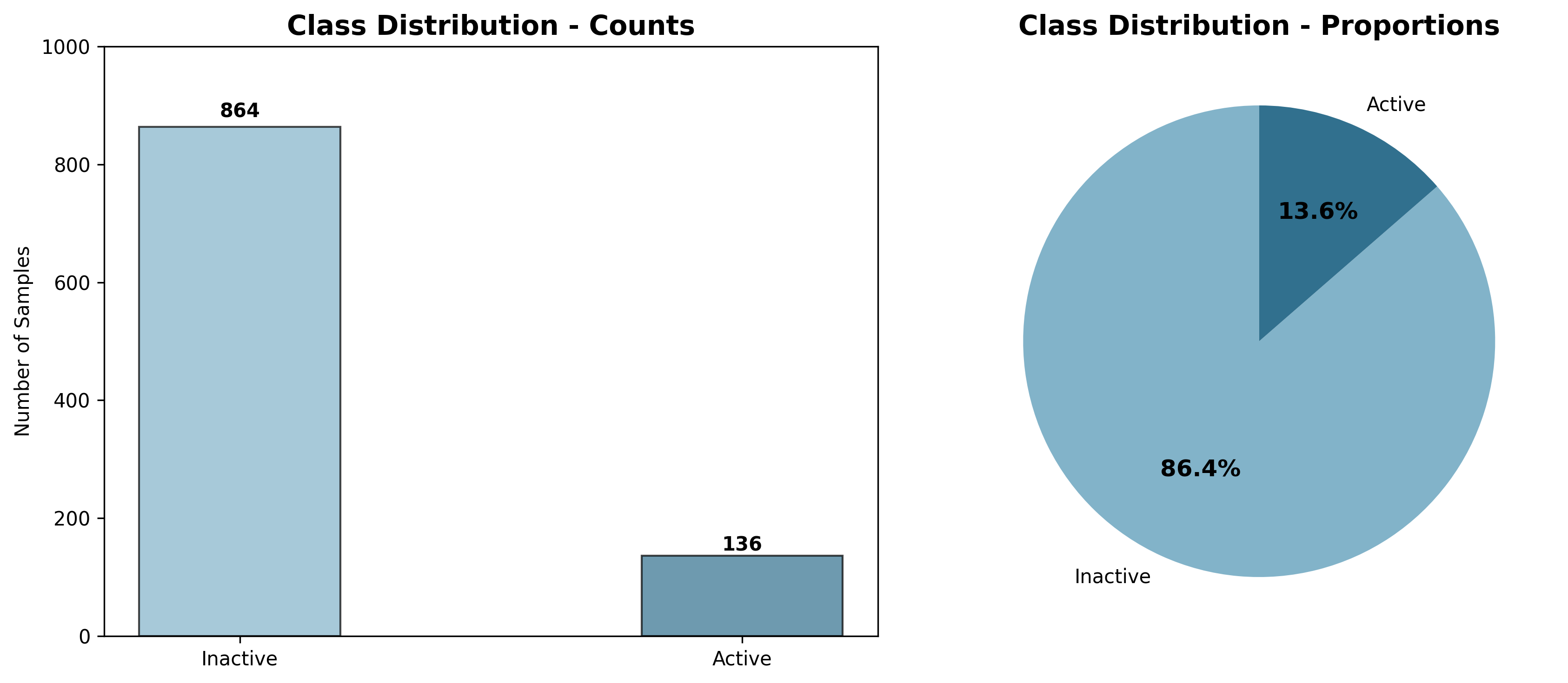
Figure 1: The severe class imbalance in our BioSynthData dataset where only ~10% of compounds are active binders.
Model Building
Now that we have some good imbalanced data, we can start building the model.
I thought that this example could work out nicely using two model types:
- A traditional random forest model.
- A more sophisticated neural network with configurable layers, batch normalization, and dropout.
For our model architecture, I’ve used PyTorch Lightning to create a modular design that separates the core model logic from metrics and evaluation. This separation is crucial because it lets us focus on the model’s actual learning without getting tangled up in how we measure its performance. Both models are wrapped in PyTorch Lightning to illustarte how traditional ML models can play nicely in this framework!
The full code for the models is available in the build_model.py file of the code-samples repository.
In short, the implementation uses an abstract base class pattern to ensure both models share a common interface for training and evaluation. The data preprocessing pipeline handles categorical encoding and converts everything to PyTorch tensors, while the training part includes proper data splitting, early stopping, and model checkpointing.
Although we wrap the models in the same framework, the way we handle the imbalanced data is quite differently: the random forest uses class weights to balance its voting mechanism, while the neural network uses weighted loss to pay more attention to the rare binding cases, as summarized in the table below:
| Model Type | Architecture | Approach |
|---|---|---|
| Neural Network | Configurable layers, batch normalization, and dropout | Weighted loss |
| Random Forest | Wrapped in PyTorch Lightning to integrate traditional ML with the framework | Class weights |
Also, the Random Forest model uses a hybrid approach, since it trains a traditional sklearn RandomForestClassifier and then transfers the learned feature importances to a PyTorch linear layer for consistent evaluation within the Lightning framework.
The key here is that the models focus purely on learning patterns in the (imbalanced) data.
Evaluation and Metrics
✨ ✨ ✨ This is where the magic happens! The evaluation and metrics module is designed to give us a clear picture of how well our models are performing, especially in the context of imbalanced data.
The evaluation module uses TorchMetrics, a powerful built-in torch library that works very nicely with PyTorch Lightning. This allows us to compute a variety of metrics during training and validation, ensuring that we get real-time feedback on our model’s performance.
Additionally, the code includes a visualization module (visualization.py) that generates plots for:
- Class distribution plots (bar charts and pie charts)
- Confusion matrix heatmaps
- ROC and Precision-Recall curves
- Metrics comparison charts
As mentioned earlier, when working with imbalanced data, we should pay special attention to precision, recall, and F1 score. The first metric we will check is accuracy, since it is the most commonly used metric. However, as we will see, accuracy can be misleading in imbalanced scenarios.
Accuracy: The Deceptive Metric
Let’s see how accuracy can be misleading in our drug discovery example. In our dataset with 1,000 compounds, where only 100 (10%) are active binders. If our model predicts all compounds as inactive, it would achieve a high accuracy of 90% (900 out of 1,000 correct). However, it would fail to identify any of the active binders, which is the primary goal of our prediction task.
Let’s look at the actual results from our models:
Model 1: Random Forest
The metrics for the Random Forest model are as follows:
Confusion Matrix for Random Forest:
True Negatives: 146, False Positives: 27
False Negatives: 25, True Positives: 2

Random Forest Metrics:
Accuracy: 0.7400
ROC-AUC: 0.5667
PR-AUC: 0.1508
Precision: 0.0690
Recall: 0.0741
F1 Score: 0.0714
The confusion matrix shows that the model correctly identified 146 inactive compounds (true negatives) but only 2 active binders (true positives). The accuracy of 74% seems reasonable, but the recall of 7.4% indicates that the model missed most of the active binders.
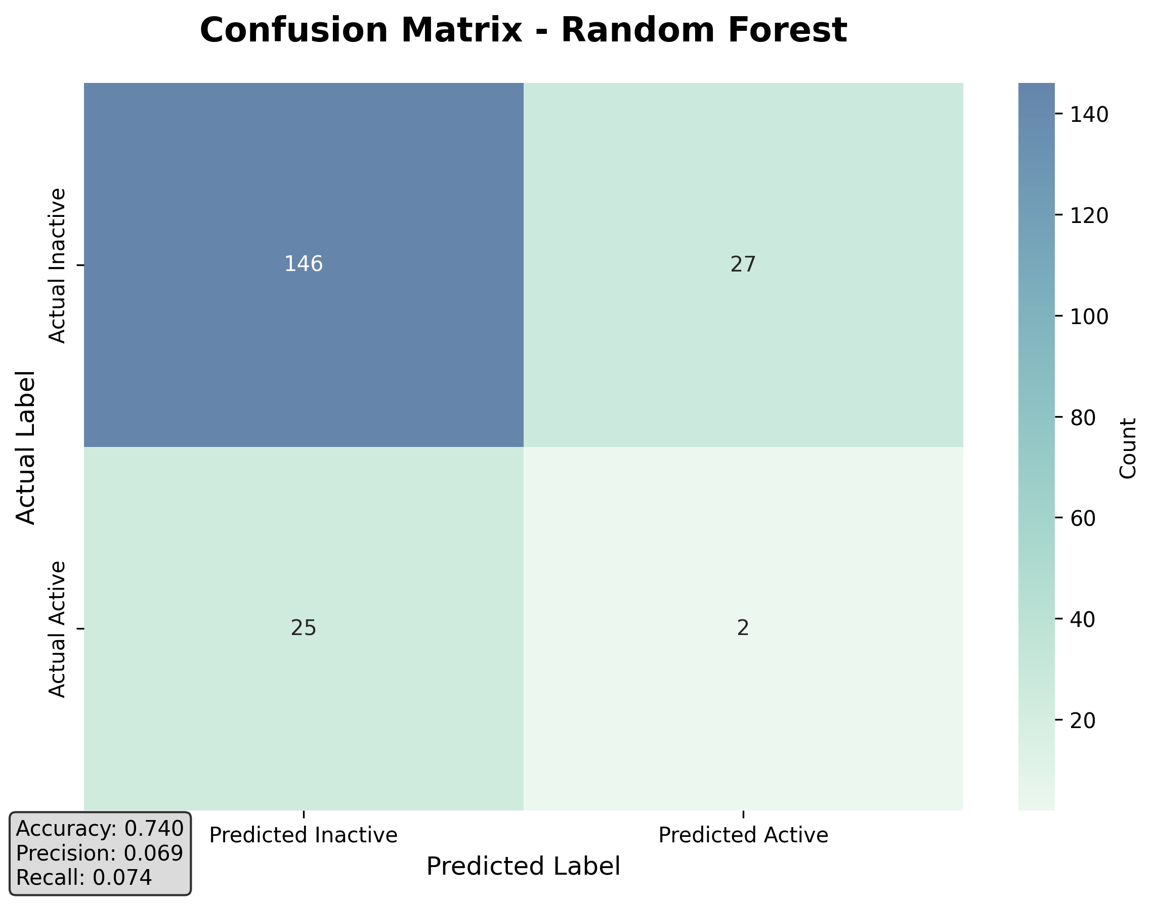
Figure 2: Confusion matrix for the Random Forest model showing the severe imbalance in predictions.
Before we continue with the next model, let’s take a moment to reflect on these results. The Random Forest model, despite its decent accuracy, is not very effective at identifying the minority class (active binders). This is a common issue in imbalanced datasets, where models tend to favor the majority class. What does the confusion matrix tell us? In drug discovery, this isn’t just an academic problem:
- ⚠️ ➖ False Negatives: Missing a promising compound could cost millions in lost revenue!
- ⚠️ ➕ False Positives: Wasting lab resources on inactive compounds delays real discoveries!
- ⚠️ False Confidence: High accuracy scores can lead to premature deployment of useless models!
This is why we need to look beyond accuracy and consider metrics that reflect our real-world goals! Now, let’s see how the Neural Network model performs.
Model 2: Neural Network
The metrics for the Neural Network model are as follows:
Confusion Matrix for Neural Network:
True Negatives: 173, False Positives: 0
False Negatives: 27, True Positives: 0

Neural Network Metrics:
Accuracy: 0.8650
ROC-AUC: 0.5778
PR-AUC: 0.1661
Precision: 0.0000
Recall: 0.0000
F1 Score: 0.0000
The confusion matrix shows that the model correctly identified 173 inactive compounds (true negatives) but failed to identify any active binders (true positives). The accuracy of 86.5% is even higher, but the recall of 0% indicates that the model did not identify any active binders at all.
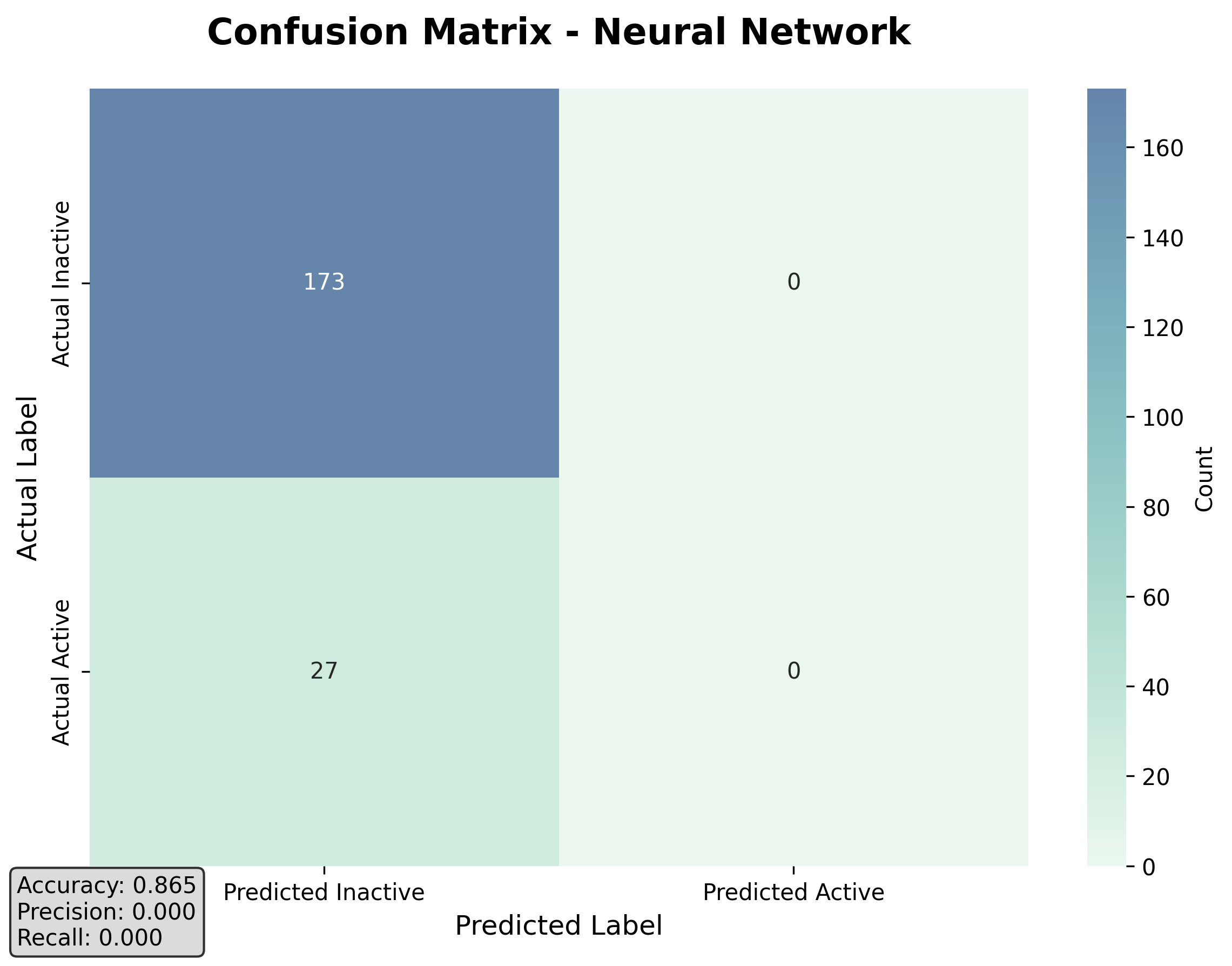
Figure 3: Confusion matrix for the Neural Network model. Despite high accuracy, it completely fails to identify active compounds.
✨ ✨ ✨ Model Comparison
The table below summarizes the key metrics for both models:
| Metric | Random Forest | Neural Network |
|---|---|---|
| Accuracy | 0.7400 | 0.8650 |
| ROC-AUC | 0.5667 | 0.5778 |
| PR-AUC | 0.1508 | 0.1661 |
| Precision | 0.0690 | 0.0000 |
| Recall | 0.0741 | 0.0000 |
| F1 Score | 0.0714 | 0.0000 |
As we can see, both models achieve high accuracy, but their ability to identify active binders is severely limited. The Random Forest model performs slightly better than the Neural Network in terms of recall and precision, but both models struggle with the imbalanced data.
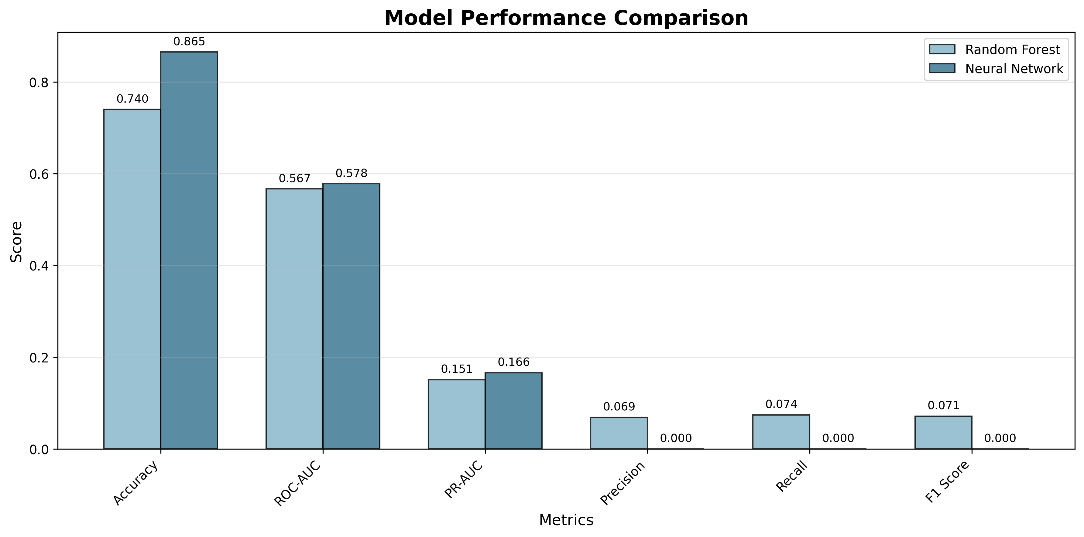
Figure 4: Side-by-side comparison of all metrics shows that both models struggle with the minority class despite high accuracy.
Hence the importance of using metrics beyond accuracy to evaluate model performance in imbalanced scenarios.
So what are the other metrics telling us?
- For precision, the metrics are low for both models, indicating that when they do predict a compound as active, they are often wrong.
- The F1 score, which balances precision and recall, is also low for both models, further highlighting their poor performance in identifying active binders.
- The ROC-AUC values are close to 0.5, suggesting that the models are not much better than random guessing.
But what about those ROC-AUC values we saw? While they look reasonable, let’s take a closer look at why they might be misleading.
ROC-AUC vs. PR-AUC: A Deeper Look
Now, popular metrics like ROC-AUC float around in machine learning talks, but here’s the catch: when your positive cases are super rare (like our 3% active compounds), ROC-AUC can make a mediocre model look impressive. That’s because it evaluates the model’s ranking ability across all thresholds, not how it handles the reality of rare positives.
Let’s look at the ROC and Precision-Recall curves to understand why ROC-AUC might not be the best metric for imbalanced data:
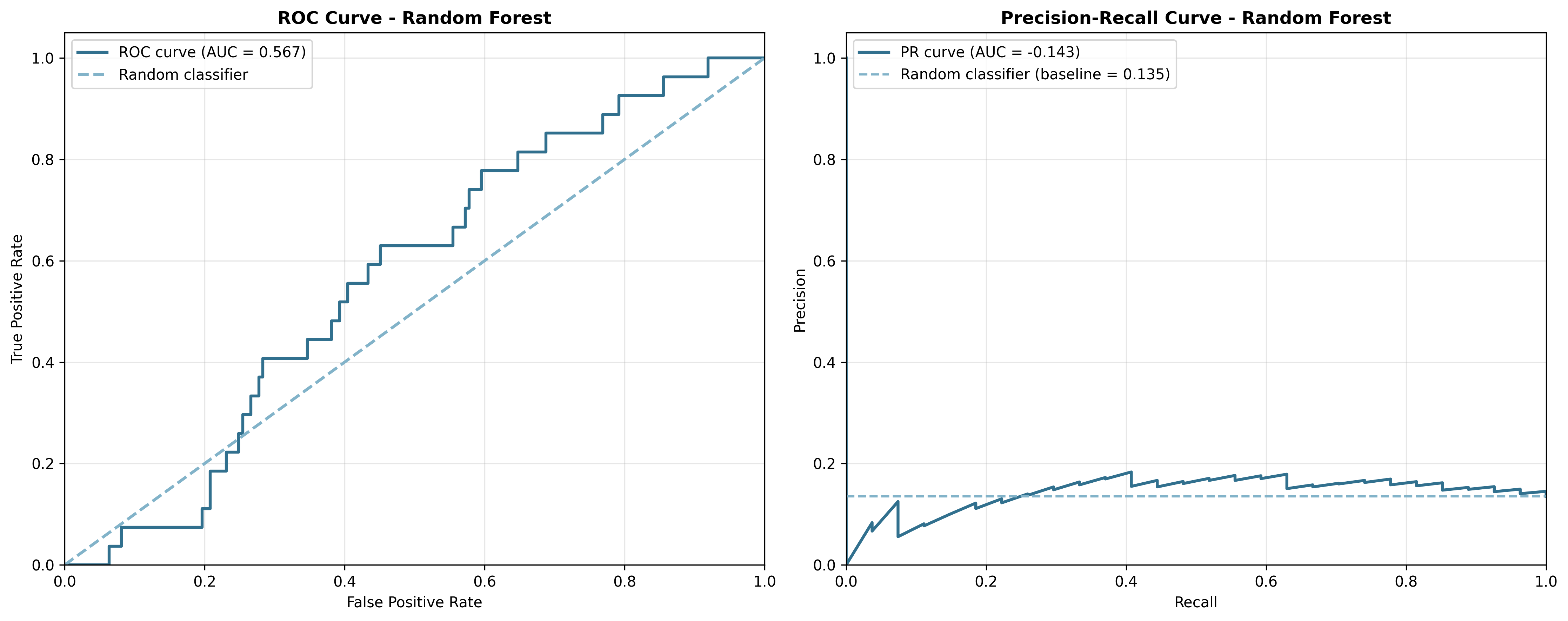
Figure 5: ROC and Precision-Recall curves for the Random Forest model. Notice how ROC-AUC (0.567) appears more optimistic than PR-AUC (0.151).
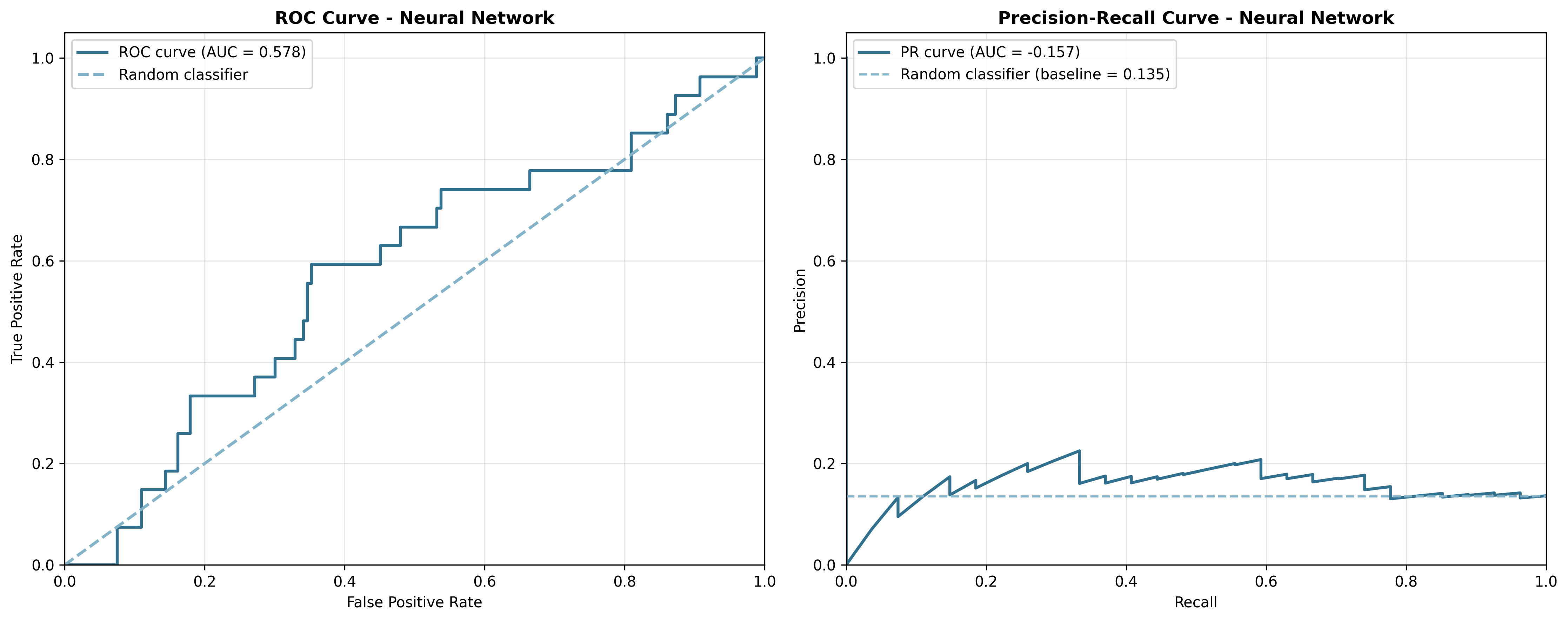
Figure 6: ROC and Precision-Recall curves for the Neural Network model show similar patterns.
The ROC curves show that both models perform only slightly better than random guessing (the diagonal dashed line). However, the Precision-Recall curves tell a more honest story. They show how poorly the models perform when we care about finding the rare positive cases.
This is where PR-AUC takes the stage. It focuses exactly on the trade-off between precision and recall. And that’s exactly what matters when active compounds are few and far between! In drug discovery, PR-AUC often tells a more honest story about your model’s performance.
Next Steps
So, what should you do next to avoid falling into the accuracy trap?
When working with imbalanced data, it’s important to go beyond accuracy as a performance measure. The first step is to examine the class distribution, since relying only on accuracy can be misleading in such cases. Instead, metrics like precision, recall, and F1-score provide a more meaningful evaluation of how well the model handles minority classes.
These metrics should be integrated directly into your evaluation pipeline, using tools such as TorchMetrics or scikit-learn to simplify computation. It’s equally important to communicate these insights with your team so that everyone understands the limitations of accuracy in imbalanced scenarios. Finally, experimenting with different decision thresholds can often improve recall while maintaining an acceptable level of precision, giving you finer control over your model’s trade-offs.
Remember: In machine learning, the right metric can mean the difference between a useful model and a dangerous one.
Key Takeaways
The accuracy trap is one of the most common mistakes in machine learning, especially in domains like healthcare, fraud detection, and drug discovery where rare events matter most.
The bottom line: When your data is imbalanced, accuracy is not just misleading. It’s dangerous! ☠️. It can give you false confidence in a model that’s actually useless for your real-world problem.
How to approach the problem?
- Always check your class distribution first
- Use metrics that reflect your business goals
- Visualize your results with confusion matrices and precision-recall curves
- Consider the cost of different types of errors in your domain
The next time you see a model with 95% accuracy, ask yourself: “What is this model actually learning?” The answer might surprise you.